Chapter 4 Results

4.1 Accosiation among indicators

Firstly, we want to see the association between our indicators in order to perform further exploratory research. We divided our variables into two parts, foundemantal(youth) education and higher education. The first part is five variables: literacy rate in youth, the complete rate in primary and lower secondary, and the out-of-school rate in primary and lower secondary. The second part for higher education is five variables: literacy rate in adults, the complete rate in upper secondary, and the out-of-school rate in upper secondary, complete 2yrs higher education rate between 25 and 29, and attend higher education rate between 18 and 22.

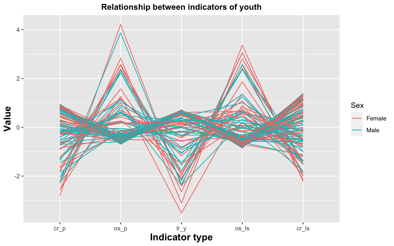
In the first parallel coordinate, we can observe that all variables have a strong relationship. The complete rate in the primary has an opposite relationship with the out-of-school rate in primary, and the out-of-school rate in primary has opposite relation with literacy in youth age. Similarly, the literacy rate has a different direction from the out-of-school rate in lower secondary but positively coordinates with the complete school rate in lower secondary.

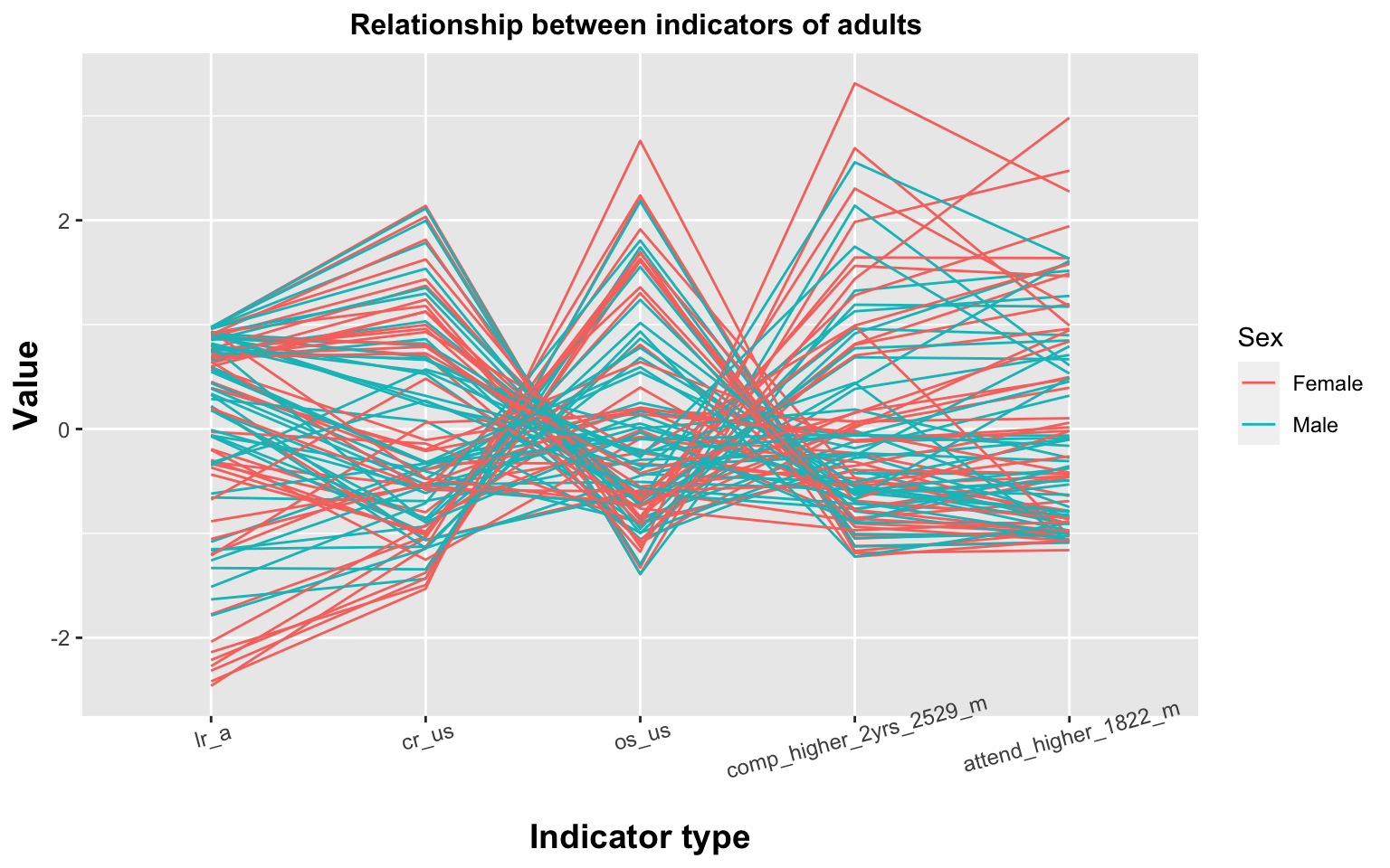
In this parallel coordinate, the out-of-school rate in upper secondary, out-of-school rate in upper secondary, and complete 2-year higher education have a clear relationship. Most adult literacy rates positively correlate with the complete rate in upper secondary. In addition, there is no such relationship between complete 2yrs higher education rates between 25 and 29 and attend higher education rates between 18 and 22.

By learning the association among all indicators, we can choose specific data combinations to learn in following sections.

4.2 Existence of gender inequalities in education

In this section, we would figure out the existence of gender inequalities in education. We would focus on the literacy rate, complete school rate, and out-of-school rate in different periods.

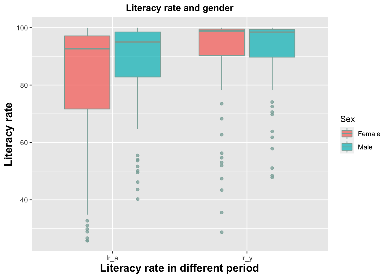
Firstly, we want to explore the literacy distribution in genders. In this boxplot, we can know the variability or dispersion of the data. the literacy rate in youth is similar in both genders. The 50% of lr_y(the literacy rate in youth) in both genders are between 90% and 100%, and the median in males and females is around 100%. More specifically, the literacy in females is slightly higher than in males, respectively 99% and 98%. There are outliers, and the minimum rate in females is 29% and 49% for males. For adults, half of lr_a(the literacy rate in adults) in different sex have different dispersion. The rates in females have larger distributions and outliers. In females, most of the rates are between 71% and 96%, while most of the data in the male are higher than in females, and 50% of male rates are between 82% and 98%. The median in males(95%) is slightly higher than 2% in females(93%).

In short, the literacy rates in youth have higher literacy rates than the literacy rate in adults in both genders. It illustrates that education has been improved a lot in both genders. In the past, literacy rates in males are higher than in females, and now literacy rates in females have better performance than in males. However, there are many countries in outliers that have a low literacy rate. We still need to improve education in those countries. We also will figure out if this situation is related to the developing regions.

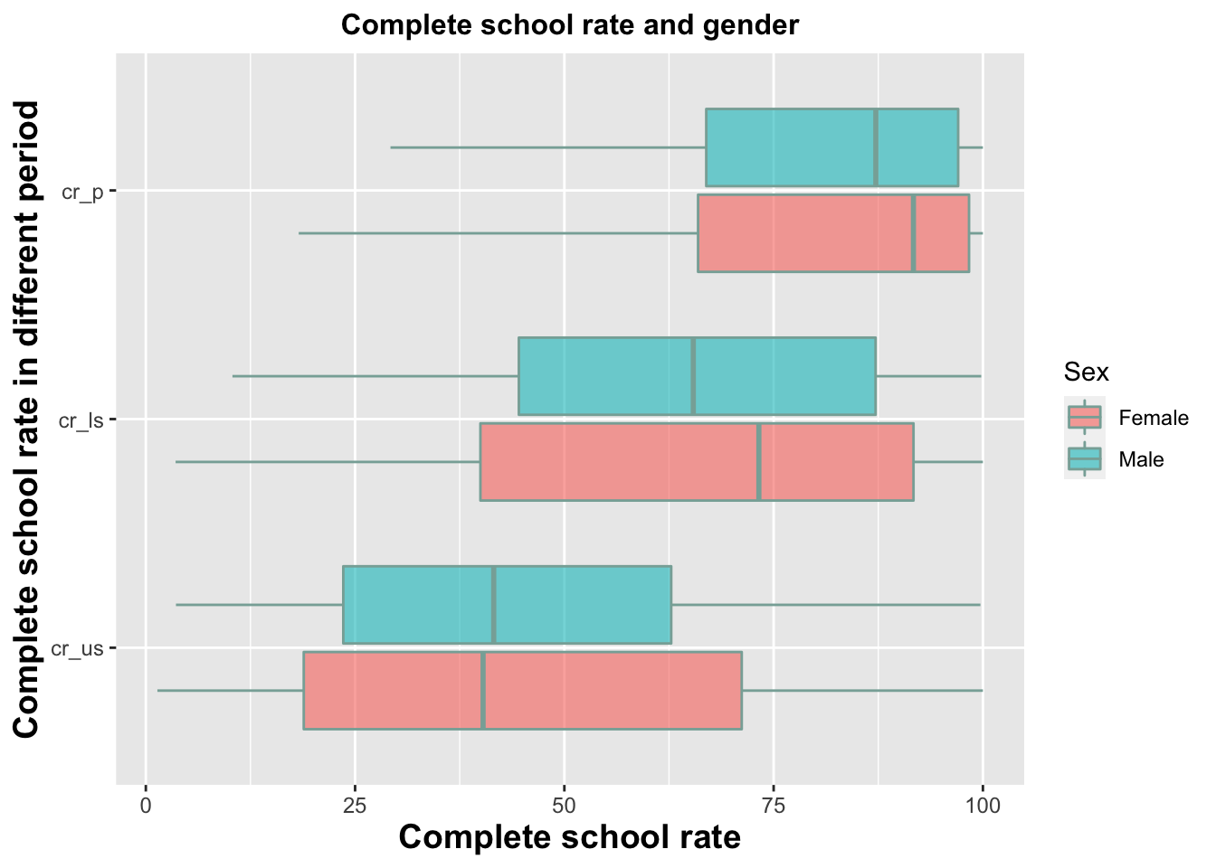
Next is to analyze the distribution of complete school rate in primary school, lower secondary, and upper secondary. In general, the complete school rate in primary school is higher than in lower secondary and then upper secondary. The maximum rates of females in each period are higher than males, but the minimum rates are lower than males. In primary school, the distribution of rates in each sex is quite similar in the interquartile range, and the median in females is higher than in males. In lower secondary, the complete school rates in females become dispersive and interquartile ranges are larger than in males. There is the same trend in the upper secondary, and the median female complete school rate is lower than males.

In short, some countries achieve higher rates, around 100%, but the trend of complete school rate from young ages to teenage ages is decreasing. The complete school rate in females have more dispersive.

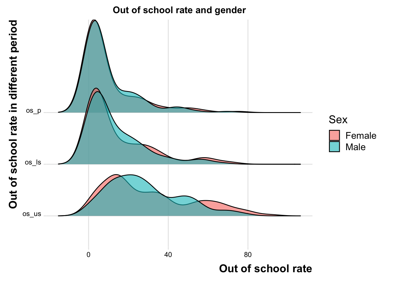
Lastly, We use the ridgeline to show the out-of-school rate in different genders. The ridgeline shows the distribution of out-of-school values for 2 groups. All graphs in primary school, lower secondary, and upper secondary show right skew, which is a good sign, and the distribution of out-of-school rates focuses on the small rates. In primary school and lower secondary, they have a parallel distribution in both genders. The out-of-school rate in lower secondary slightly move to the right. The female rates in lower secondary are higher than male rates in the peak, and then the male rates are higher than females. For upper secondary, it is clear to observe that the distribution moves to the right a lot, and the rates at peak become larger around 20%.

In this chapter, we can observe that education of different gender still exists bias and inequality. The above graph illustrates that some of the female median values about the complete school rate are higher than males, but the mean values of females are lower than males. The total education data in females have a large distribution range, and there are obvious gaps and disparities between the complete school rate in females. Next step, we want to focus on education differences between males and females in certain countries.

4.3 Possibility of gender discrimination for countries with education underachievements

In the above section, we validate that gender discrimination in education still exists. Therefore, we want to explore whether it is a general pattern or only certain countries sit in this situation by visualizing the primary out-of-school rate, mean years of education, and higher education attendance rate so that both fundamental and higher education can be learned.

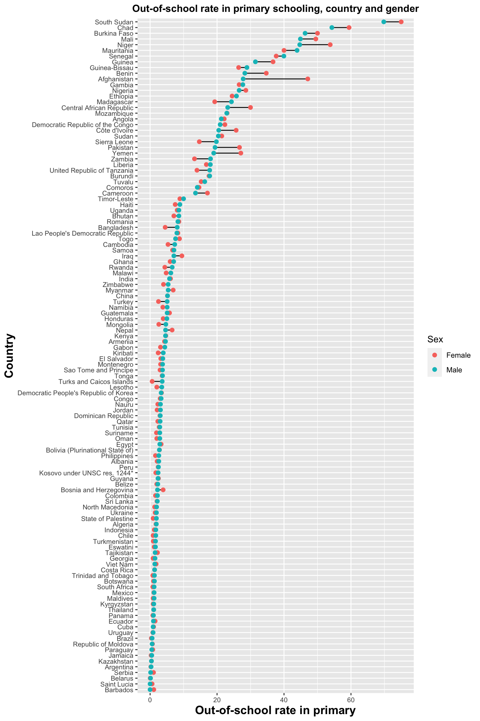
In this plot, we explore the out-of-school rate of primary schooling. It is clear that when the rate becomes higher than 5%, female rates become higher than male rates, which indicates that females seem to have less opportunity of going to primary school than males in those countries with higher out-of-school rates.

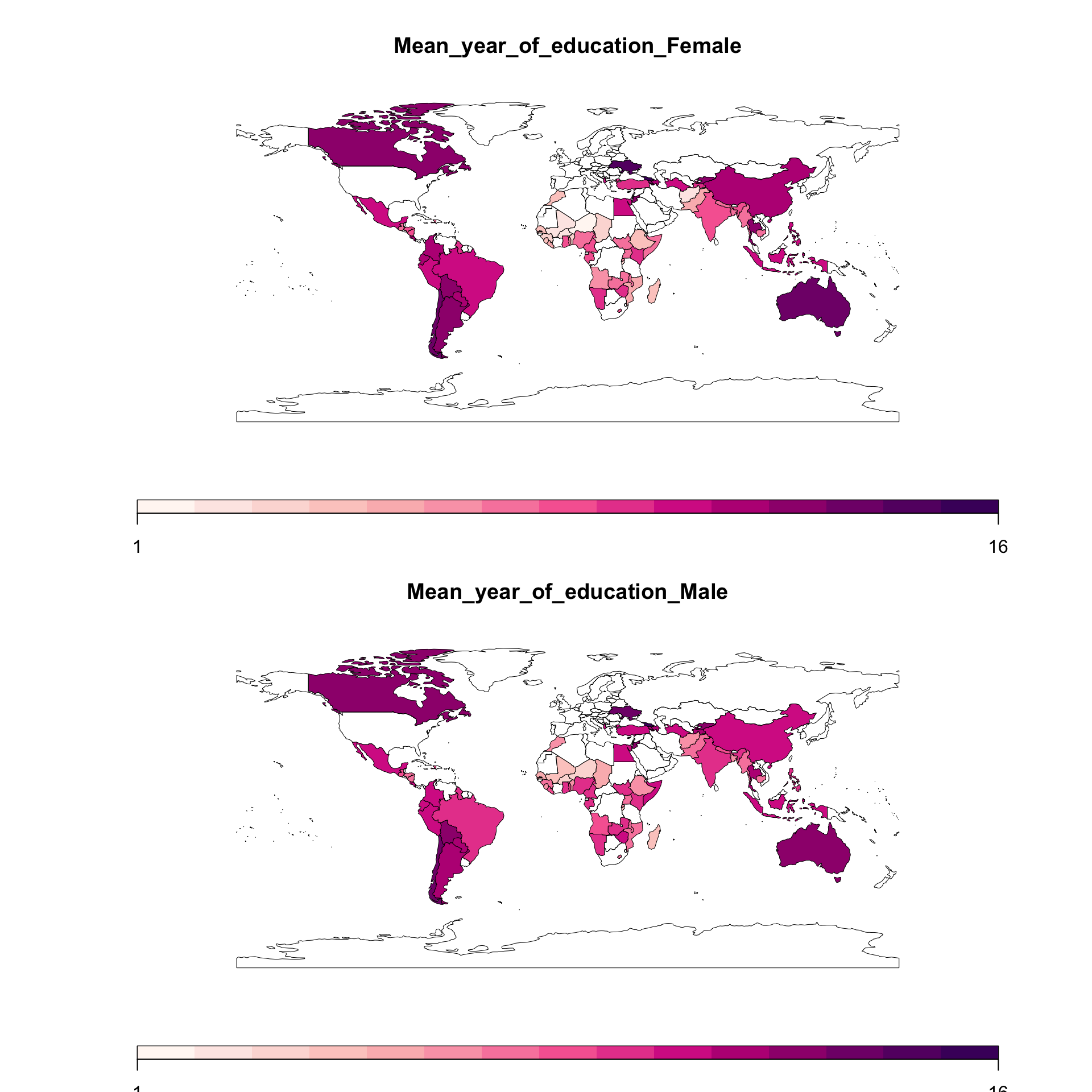
The indicator named”eduyears_2024_m” is th average number of years of schooling attained for the age group 20–24 years.These world maps show that most countries have no big differences between male and female figures. To study how the two figures are different, an additional map is visualized for plotting the difference between males and females.

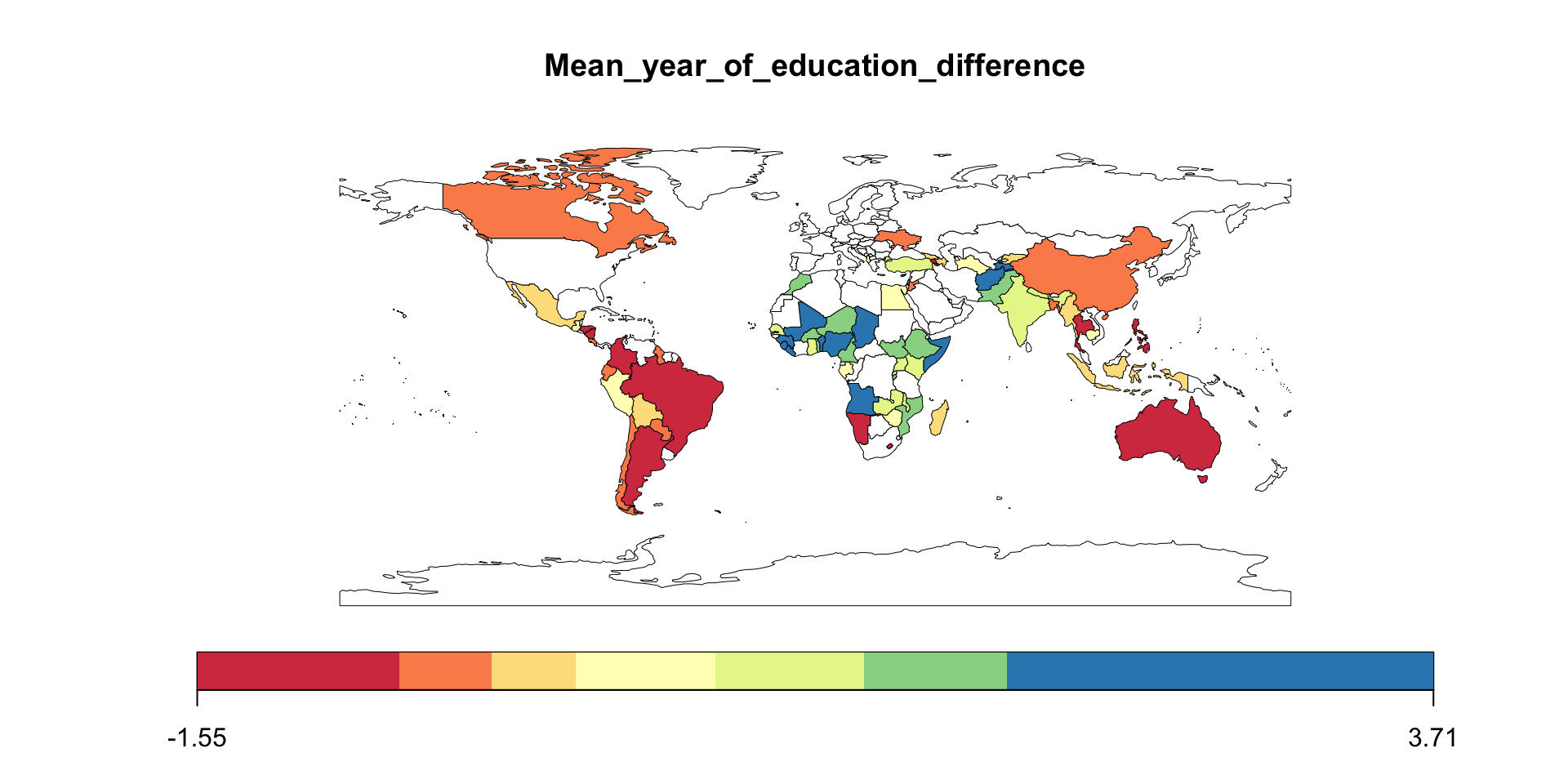
In this map, a diverging color palette is used. In detail, light yellow indicates a neutral difference. The warm colors indicate that female is higher than the male, while the cold colors indicate the opposite. We observe that the region with males higher than female is mainly in Africa and West Asia. Then we use a bar chart to explore this pattern more.

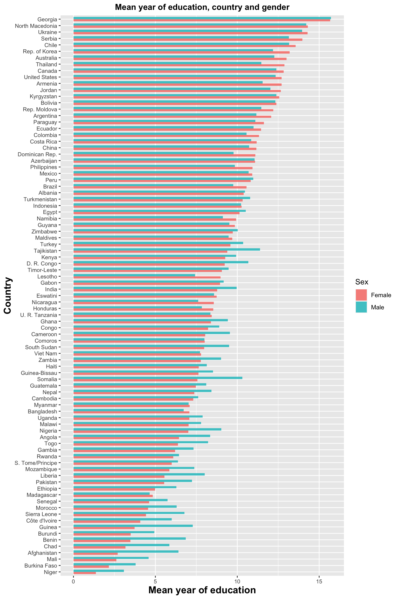
In this bar chart, it shows trend that the fewer years of education, the more the male figure is higher than the female figure. Some outliers with at least 7.5 years of schooling but significantly higher male averages than female averages are detected: Tajikistan, D. R Congo, Kenya, Somalia, South Sudan, etc.

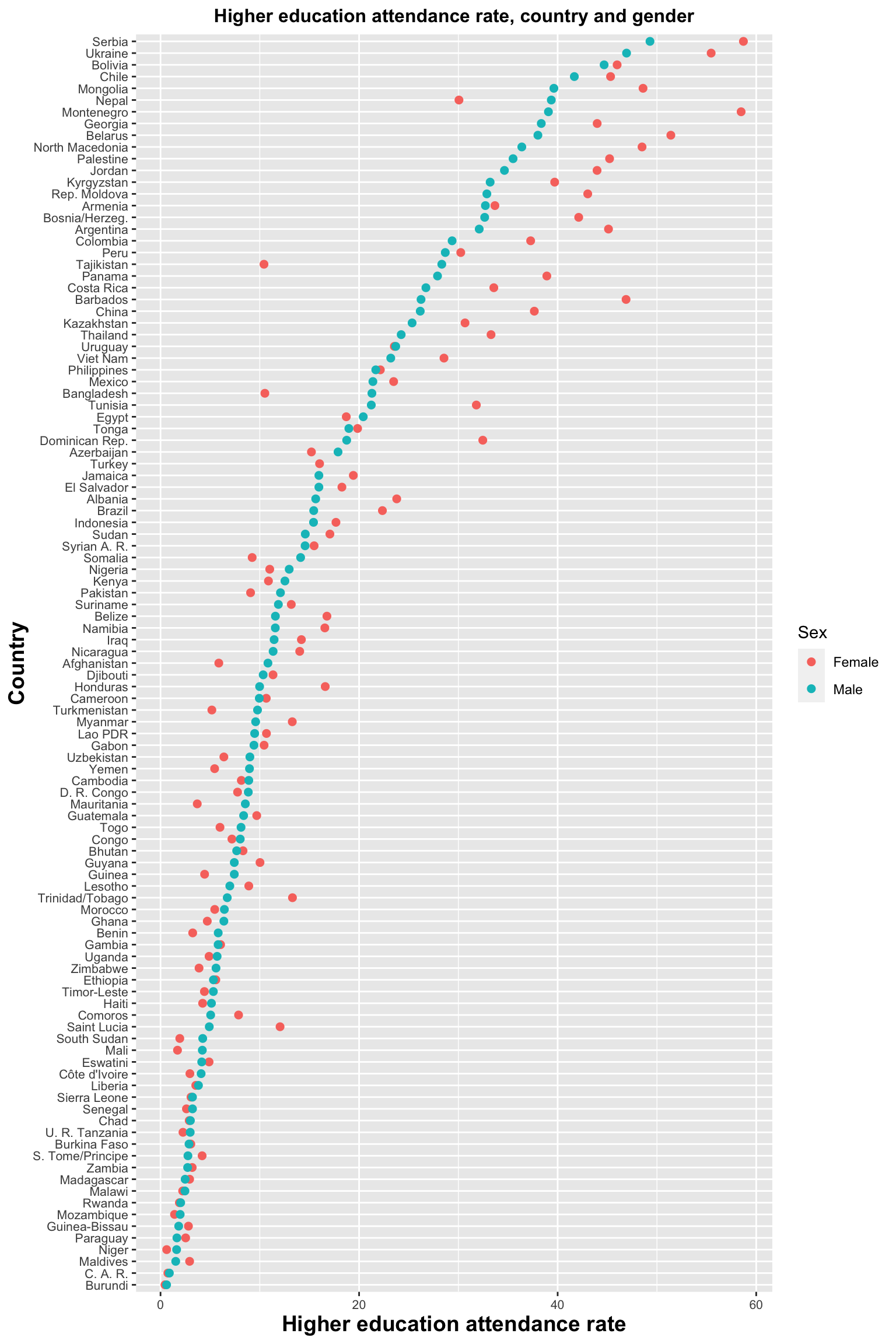
In this Cleveland plot, for countries with higher education attendance rates over 10%, more countries have female rates higher than male rates. In comparison, countries with below 10% rates are more to have higher male rates than female rates, even though the difference is not as big as the mean education year. This not only helps indicate that countries with a low higher education attendance rate are having gender inequality problems but also illustrates that in those countries with high levels of education, females own better figures in higher education.

Meanwhile, there are also some outliers, such as Nepal, Tajikistan, Bangladesh, Kenya, Somalia, etc. They have higher male rates but with decent higher education attendance rate.

It is worth mentioning that outliers from the two plots are highly overlapped. And most outlier countries lie in the below-average cluster for at least one plot. This situation may also involve other aspects. Therefore, we would investigate the influence of the financial and development level of countries.

4.4 Relationship among development level, education achievement and gender

The above section demonstrates that countries with education underachievement have more possibility of remaining gender preconceptions. In this section, how development level, education level, and gender is related is explored by visualizing tertiary completion rate and mean year of education.

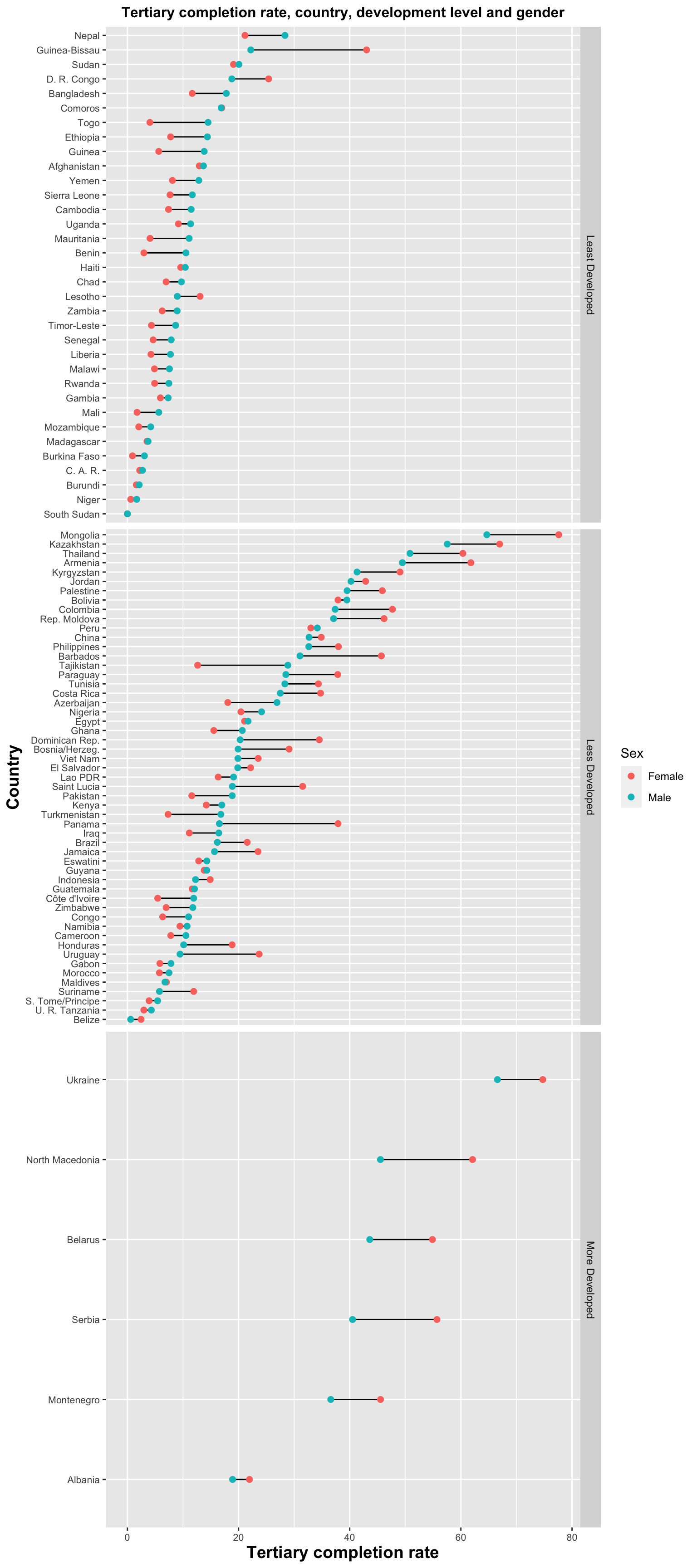
After taking development into account, we discover from this Cleveland plot that, in general, least developed countries seem to have lower tertiary completion rates, and rates of most more developed countries are above 40%. Moreover, there is more observation that male rates are much higher than female ones in the least developed regions. And our outliers from the previous section mostly lie in this facet. It validates our hypothesis that lower-developed regions are more likely to have unsatisfied education situations and gender discrimination. On the other hand, unlike indicators of fundamental education, this plot of tertiary completion rate presents that for most countries in more developed and less developed facets, female rates are higher than male ones, implying again that female has good performance in higher education.

We want to use mean year of education as indicator for further exploration. We categorized the mean year of education into three cuts (low(<6), middle(6-10), and high(>10)) and visualized its relationship with development level and gender using Mosaic plot.

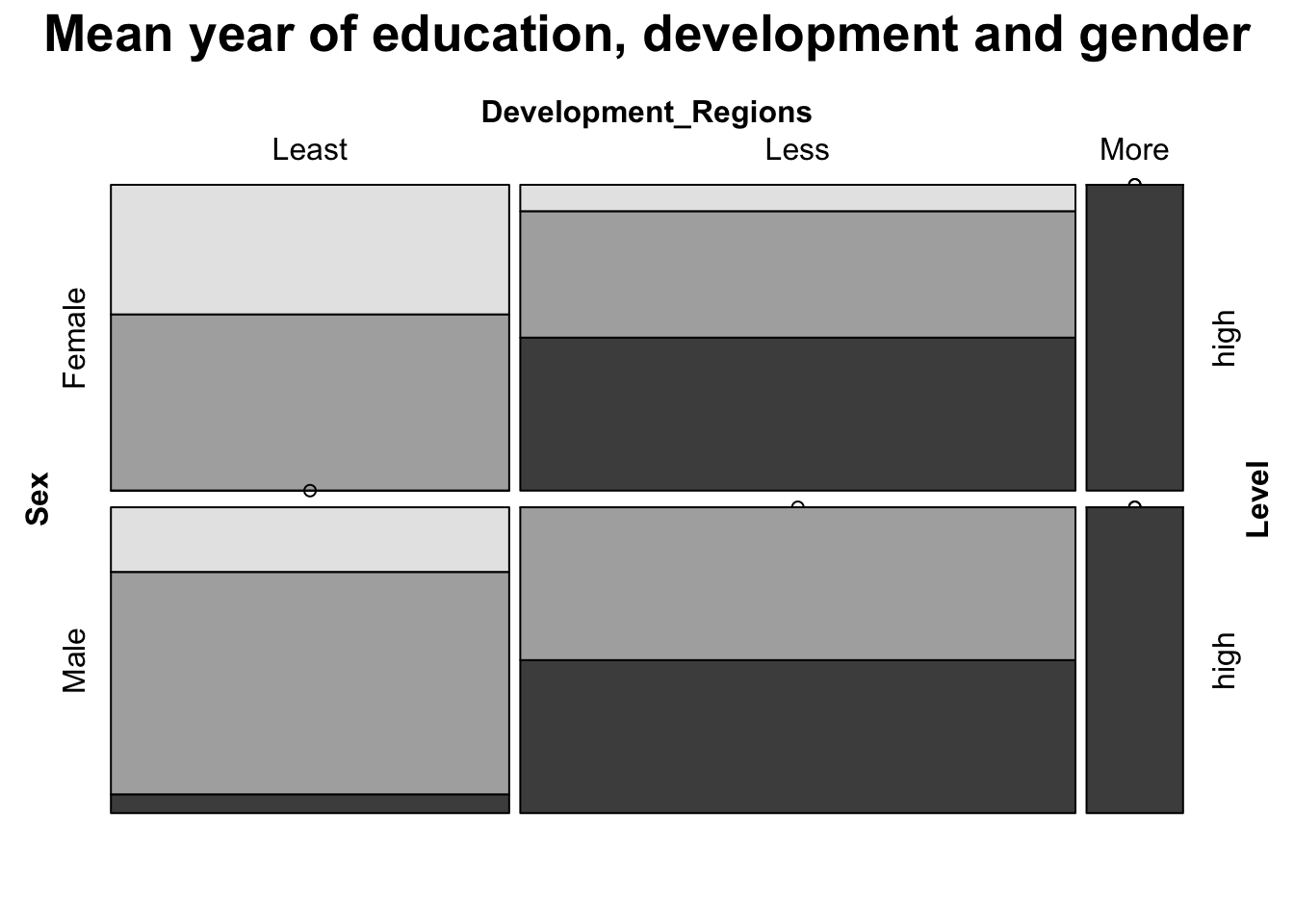
In this plot, the lightest shade is low for level of mean year of education while the darkest is high. From the Mosaic plot, there are several noticeable patterns. Firstly, female in the least developed countries only have low and middle figures, which mean they barely get educated for more than 10 years. For females in less developed regions, the vast majority of them get medium and high figures while the high proportion is slightly higher than the medium. Secondly, the majority of male in the least development regions lies in the middle region. Only a very small proportion can receive education for more than 10 years. Males in less developed countries only have middle and high figures. Finally, the regions of more developed countries are deterministic no matter the gender. Everyone from more developed countries can receive at least 10 years of education, which represents adequacy and equal distribution of educational resources.

Therefore, we prove that countries with poor education performances and more severe gender stereotype situations are more likely to be less developed.